The most commonly used seismic method is seismic refraction.
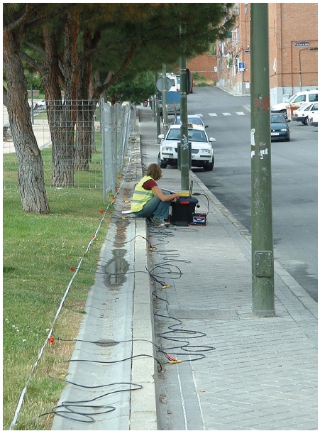
Longitudinal sections equipped with an array of sensors (geophones) are repeated at regular, known intervals. Energy released by a “shot” (usually a blow with a 6–8 kg hammer) reaches the sensors, generating a seismic disturbance recorded on a seismograph. The sections are usually 25–100 m long, and the geophones are placed less than 5 m apart, to guarantee detailed results. There are usually at least three shot points, at the beginning, middle and end of each profile. For profiles more than 60 m long, five shot points would be used.

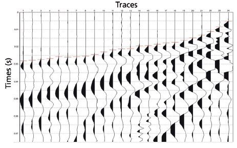
The time the elastic waves take to reach the geophones is measured to give the propagation velocity value and thickness of the different materials they pass through. Figure 1 shows one type of seismograph, and Figure 2 shows an example of a seismogram.

The travel time between the precise moment of the shot and the arrival of the first disturbance is measured for each geophone. The first waves to arrive are direct waves, but at a certain point (the critical distance), the refracted waves travelling through the lower levels of the substratum arrive first. The longer distance travelled by these waves is compensated by their greater velocity (Figure 3).

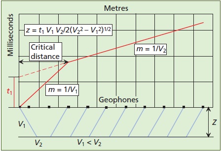
The travel time graph is the linear function relating the arrival time of the first wave with the distance it has travelled.
Each refractor has a travel time graph and the slope and ordinate at origin of each arrival, are used to calculate the velocity of the medium and the depth at which the refraction surface is found (Figure 4). The line passing through the origin to the arrival of the refracted rays corresponds to the arrival of direct waves.

Refractors are not usually flat and so the arrival times of the signal from the refractor need not be perfectly aligned. There are several methods for obtaining the depth and velocity below each geophone, based on deviations from the theoretical curve that are observed for arrival times at a geophone when the outward time is measured and return time is read (Figure 5).

The transmission velocity of seismic waves is a good indicator of the geotechnical characteristics of materials.
Tables of velocities for different rock materials frequently appear in the literature, although there is a significant divergence of velocity values. This is due to the variability in lithology or internal structure, to the percentage of pores or cavities, and to fluid saturation (Figure 6). As the materials disintegrate and the degree of alteration increases, the velocity is reduced.

The degree of weathering of rocks is clearly a factor conditioning seismic wave propagation velocity; an unaltered rock such as a fresh granite may have a velocity of 5,000 m/s, but if it is highly altered this may drop to as low as 1,000 m/s or less.
Seismic refraction is used in geological engineering to determine the depth of made ground, superficial drift, substratum structure, material rippability and borrow pit volumes.